How researchers take massive models from research labs to production - optimizing for faster inference, lower cost, and broader deployment across servers, edge devices, and beyond.
The Gap Between Research and Reality
In 2012, AlexNet won ImageNet with 60 million parameters and needed two NVIDIA GTX 580 GPUs to train. A decade later, GPT-3 has 175 billion parameters. GPT-4's architecture has not been officially disclosed, but training costs are estimated in the tens to hundreds of millions of dollars. The compute budget for frontier models has grown by roughly 4- 5 orders of magnitude in ten years - and with it, the cost of running them.
Inference is now a serious economic problem even before you consider mobile devices. Serving a single 70B parameter model in float32 requires ~280 GB of GPU memory - roughly four A100 80GB GPUs just to load the weights, before a single user request arrives. At scale, inference compute costs can exceed training costs within months of a model's release. The field has responded with a deep and compounding set of techniques to make models smaller, faster, and cheaper to run - without losing what makes them good. The pace of progress is striking: Gemma 4 E2B can now run on phones, signaling that edge inference is becoming increasingly viable.
The journey from a research model to a deployed one typically flows through five stages: efficient architecture design, neural architecture search, pruning, knowledge distillation, and quantization. Each attacks the problem from a different angle. Most production deployments combine several.
Stage 1 – Architecture Design: Efficiency as a First Principle
The most impactful efficiency gains don't come from compressing a bad model, they come from designing a good one from the start. The standard building blocks of deep learning (full convolutions, dense attention) are computationally expensive relative to what they actually need to compute.
Depthwise Separable Convolutions
In 2017, Howard et al. published MobileNets, factorizing a standard convolution into two cheaper operations. A standard convolution with a K×K kernel, M input channels, N output filters, and an output feature map of spatial resolution W_out × H_out costs K² × M × N × W_out × H_out multiply-accumulate operations - one for each kernel element, across every input channel, for every filter, at every output spatial location. Depthwise separable convolution splits this into a per-channel depthwise step plus a 1×1 pointwise step, often reducing computation by several times (commonly around 8× for a 3×3 kernel, depending on channel dimensions).
MobileNetV1 achieved 70.6% top-1 ImageNet accuracy with 4.2 million parameters and 569 million multiply-adds. VGG-16 reached 71.5% accuracy using 138 million parameters and 15.5 billion MAdds - 33× more computation for a 0.9% accuracy difference.
In 2018, MobileNetV2 added the inverted residual block: expand channels, apply depthwise convolution, project back down with a linear (no-ReLU) bottleneck. This “expand → depthwise → project” template strongly influenced many subsequent efficient CNN architectures, becoming a widely adopted pattern for building compute-efficient models.

Grouped Query Attention
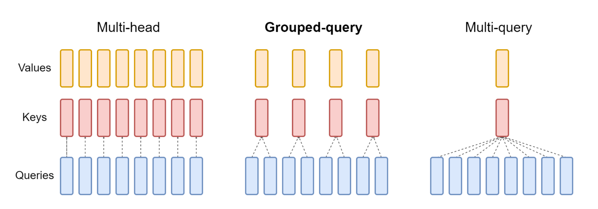
In transformer models, the attention mechanism is the primary bottleneck at inference time - specifically, the KV cache. Standard multi-head attention stores a key and value vector per head per token, which grows linearly with sequence length and number of layers. For a 70B model generating long sequences, the KV cache alone can consume tens of gigabytes.
Grouped Query Attention (GQA, Ainslie et al., 2023) addresses this by sharing key and value heads across multiple query heads. With 8 query heads sharing a single KV head (GQA-8), you reduce KV cache memory by 8x with minimal impact on model quality. GQA is now standard in production LLMs: LLaMA 3 and Mistral use it. It directly reduces inference memory and increases the batch sizes a server can sustain - which is the primary lever for reducing per-token serving cost.
Sliding Window and Dilated Attention
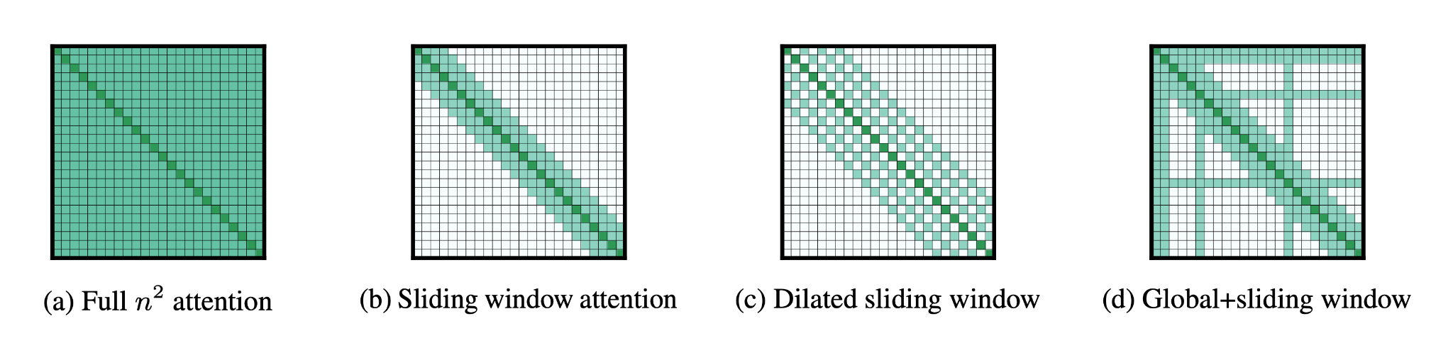
Full self-attention has `O(n²)` complexity in sequence length - fine for short sequences, prohibitive for long ones. Two complementary ideas address this. Sliding window attention restricts each token to attending only to the W most recent tokens per layer - Mistral 7B (Jiang et al., 2023) used `W=4096` in a production model, bounding per-token compute while still propagating information from beyond the window through successive layers. Dilated sliding window attention extends this by spacing attended positions at a fixed interval rather than attending to consecutive tokens, giving a wider effective receptive field without increasing the window size - analogous to dilated convolutions in CNNs. Longformer (Beltagy et al., 2020) studied both patterns systematically, showing that combining local window attention with a small number of global tokens recovers most of the representational power of full attention while reducing complexity from `O(n²)` to `O(n)`, making long-sequence processing practical at inference time.
Stage 2 – Neural Architecture Search: Letting Machines Design Machines
Manual architecture design has practical limits when targeting diverse hardware. Intuition developed on CPUs and GPUs does not always translate cleanly to NPUs, custom ASICs, or emerging accelerators, where memory access patterns, operator fusion, and parallelism constraints can dominate performance. As a result, models with fewer FLOPs can still run slower on specific silicon. Neural Architecture Search (NAS) addresses this by automating architecture design against explicit hardware objectives.
MnasNet – Hardware in the Loop
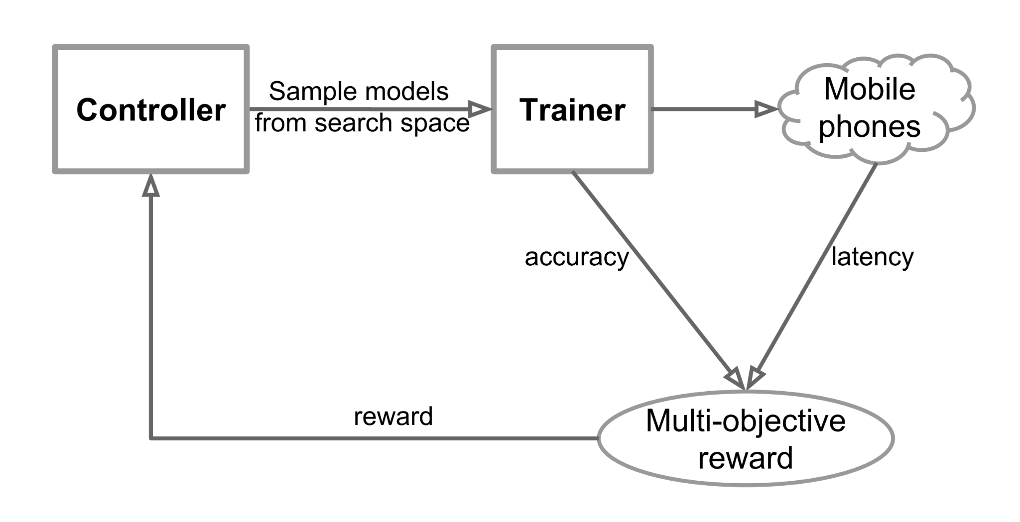
Google’s MnasNet (Tan et al., 2019) was among the first large-scale NAS systems to optimize architectures directly against measured on-device latency. The objective combined accuracy and latency, defined as `ACC(m) × [LAT(m) / T]^w` where LAT was obtained by deploying candidate architectures to a physical device and timing their execution. The search used reinforcement learning: a controller proposed architectures, they were trained on a proxy task, deployed to hardware, and real latency measurements were fed back as the reward signal.
On target mobile devices, MnasNet discovered architectures that were significantly faster than MobileNetV2 at comparable accuracy, using heterogeneous layer-wise operations that would have been difficult to design by hand.
EfficientNet – Compound Scaling
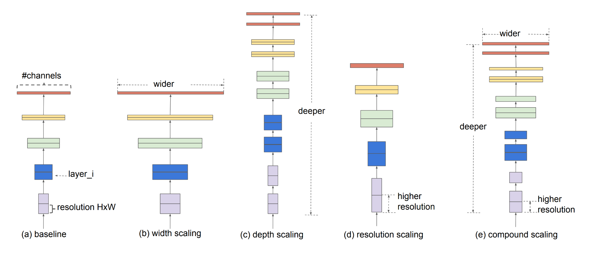
EfficientNet (Tan and Le, 2019) asked a simple but powerful question: given a fixed compute budget, how should model capacity be allocated across width, depth, and input resolution? Rather than scaling a single dimension arbitrarily, they used NAS to identify a balanced baseline and empirically derived a compound scaling rule. For their baseline model, a 2× increase in FLOPs corresponded to scaling depth by ~1.20×, width by ~1.12×, and resolution by ~1.15× simultaneously.
This compound scaling coefficient φ generated an entire model family from a single NAS-found baseline (EfficientNet-B0, 5.3M parameters, 77.1% top-1). EfficientNet-B7 reached 84.3% top-1 accuracy with 66M parameters, outperforming much larger models. EfficientNet-B0 achieved accuracy comparable to ResNet-50 with several times fewer parameters and an order of magnitude lower compute.
The key insight was not the specific architecture, but the scaling rule itself: once you have a strong base model, there is a principled way to scale it up or down to meet different compute budgets.
Once-for-All – One Search, Many Targets
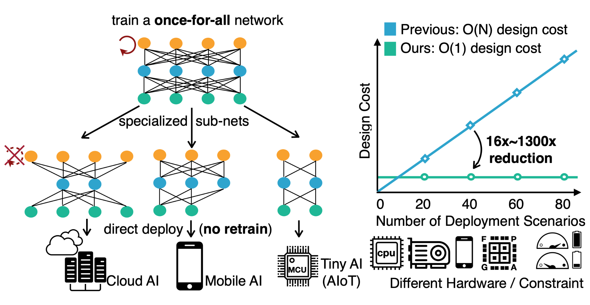
A practical limitation of hardware-aware NAS is cost. MnasNet-style searches required thousands of GPU-hours per target device, which becomes prohibitive when deploying across many hardware platforms.
Once-for-All (Cai et al., 2020) addressed this by training a single over-parameterized “supernet” that contains many possible sub-networks. During training, a sub-network is sampled at each iteration and only its corresponding weights are updated. After training, specialized sub-networks for new hardware targets can be extracted using a lightweight evolutionary search- typically requiring only a few GPU-hours and no retraining, since the weights are already calibrated. This approach dramatically reduced per-target search cost while achieving performance comparable to individually NAS-optimized models.
Stage 3 – Pruning: Removing the Dead Weight
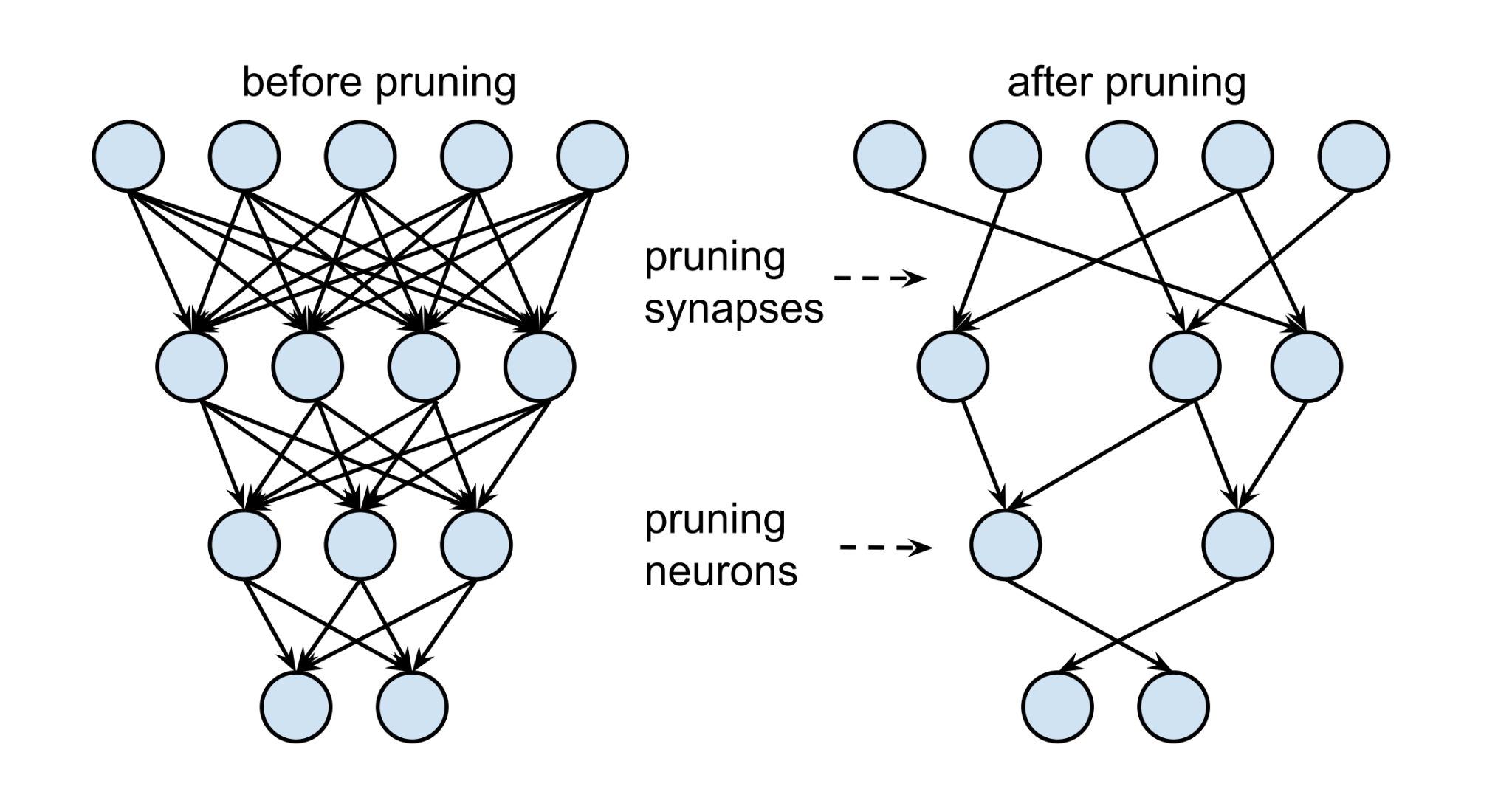
Once a model is trained, not all of its parameters contribute equally to performance. The lottery ticket hypothesis (Frankle and Carbin, 2019) captures this intuition by showing that large networks can contain sparse sub-networks which, when trained from the same initialization, are capable of reaching accuracy comparable to the full model. Pruning methods aim to identify and remove parameters that contribute least to the final output.
Unstructured pruning removes individual weights, typically by magnitude. Han et al. (2015) demonstrated substantial compression on AlexNet with minimal accuracy loss by combining iterative pruning with quantization and entropy coding. However, unstructured sparsity is difficult to exploit on standard hardware: unless the sparsity follows specific patterns (such as NVIDIA A100’s 2:4 structured sparsity), highly sparse weight matrices often still execute largely dense operations on GPUs, yielding limited speedups in practice.
Structured pruning removes entire channels, attention heads, or layers, producing a smaller dense model that runs efficiently on existing hardware without specialized support. For large language models, this form of pruning is generally far more practical for real-world deployment.
SparseGPT (Frantar and Alistarh, 2023) introduced a one-shot pruning method for large pretrained transformers, achieving 50–60% unstructured sparsity on models up to tens of billions of parameters. The method uses a second-order approximation derived from the Hessian to compensate for removed weights, requires no gradient computation, and can be applied post-training- making it suitable for models where full retraining is prohibitively expensive.
Wanda (Sun et al., 2023) further simplified large-model pruning by scoring weights using |weight| × ‖input activations‖₂ in a single forward pass and pruning the lowest-scoring parameters. This approach achieves sparsity levels comparable to SparseGPT with dramatically lower computational overhead, making large-scale pruning accessible without specialized second-order optimization machinery.
Stage 4 – Knowledge Distillation: Teaching a Small Student
A trained neural network’s output contains more information than the correct label alone. When classifying a cat, the model also assigns non-zero probabilities to related classes like “tiger” or “leopard,” producing a soft distribution that encodes similarity structure which a one-hot label discards. Knowledge distillation (Hinton, Vinyals, and Dean, 2015) exploits this additional signal.
A common distillation objective is `L = α · CE(y, p_student) + (1 − α) · KL(p_teacher,τ ‖ p_student,τ)` where temperature τ (typically in the range of ~2–10) softens both teacher and student distributions to amplify information in low-probability classes. The exact formulation and weighting vary across implementations.
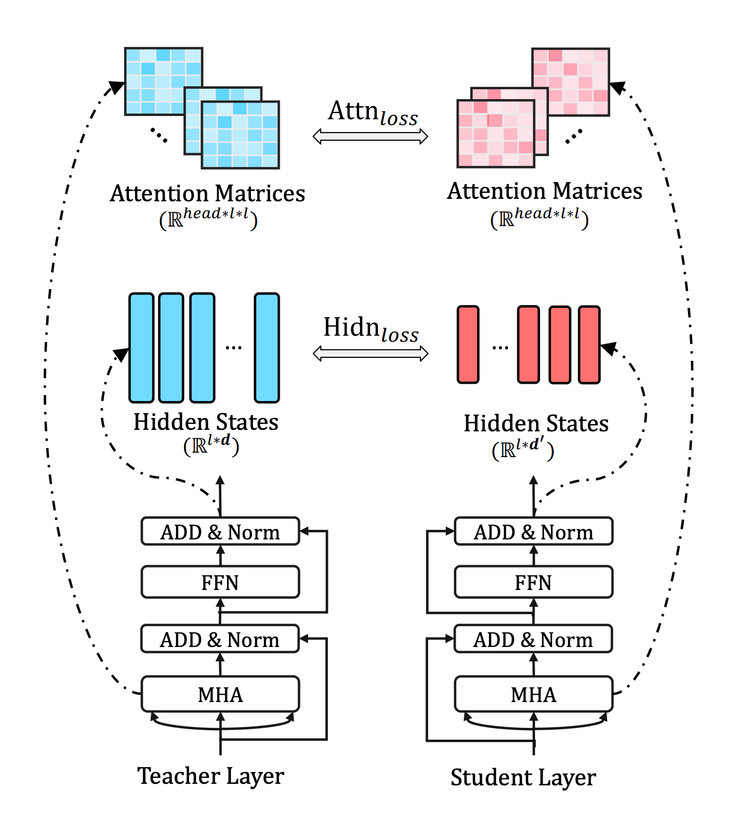
DistilBERT (Sanh et al., 2019) compressed BERT-base (110M parameters, 12 layers) into a 6-layer, 66M-parameter student using a combination of soft-label distillation, intermediate hidden-state alignment, and attention-level losses. The resulting model retained roughly 97% of BERT-base performance on GLUE while being ~40% smaller and significantly faster at inference.
TinyBERT (Jiao et al., 2020) extended this idea by applying distillation during both pre-training and task-specific fine-tuning. This multi-stage approach achieved performance close to the teacher model while delivering substantially faster inference, demonstrating that pre-training-time distillation compounds with downstream task distillation.
For vision transformers, DeiT (Touvron et al., 2021) showed that a ViT trained from scratch on ImageNet- without large-scale external pretraining- could reach competitive accuracy by distilling from a CNN teacher. In this setting, the CNN’s spatial inductive biases were transferred through the teacher’s softened outputs rather than architectural constraints.
Distillation also scales to large language models. LLaMA 3.2 1B and 3B (Meta, 2024) were produced via a prune-then-distill pipeline: starting from a larger LLaMA 3.1 8B model, structured pruning reduced capacity, followed by distillation-based fine-tuning to recover quality. The smallest variants outperform many larger baselines on selected benchmarks- performance not achievable through pruning alone.
Stage 5 – Quantization: Shrinking the Numbers Themselves
The techniques above reduce the number of parameters or operations. Quantization instead reduces the precision of each number. A standard weight stored in FP32 uses 32 bits; INT8 uses 8 bits (4× smaller), INT4 uses 4 bits (8× smaller), and INT2 uses 2 bits (16× smaller). For a 7B-parameter model, this translates approximately to:
- FP32: ~28 GB
- BF16: ~14 GB
- INT8: ~7 GB
- INT4: ~3.5 GB
- INT2: ~1.75 GB
Post-training quantization (PTQ) converts a trained floating-point model using a small calibration set to estimate activation ranges, without retraining. INT8 PTQ typically incurs negligible accuracy loss for vision models. For LLMs at INT4, however, naive PTQ leads to significant degradation, motivating more sophisticated methods.
GPTQ (Frantar et al., 2022) quantizes weights layer-by-layer, compensating for quantization error by updating remaining full-precision weights using a second-order approximation of the layer output. This enabled 4-bit quantization of very large transformer models within hours on a single GPU, making inference feasible on hardware where full-precision models would not fit.
AWQ (Lin et al., 2023) observed that weight importance is highly non-uniform: weights connected to large activations disproportionately affect model output. By selectively protecting a small fraction of weights from aggressive quantization, AWQ achieves better perplexity than GPTQ at comparable bit-widths, with lower computational cost and no Hessian computation.
GGUF, the format underlying llama.cpp, popularized per-layer mixed-precision quantization- using higher precision for embeddings and attention layers and lower precision for feed-forward blocks. This flexibility allows practitioners to meet strict memory budgets while minimizing accuracy loss, enabling large-model inference on consumer hardware.
BitNet b1.58 (Ma et al., 2024) pushed quantization to the extreme by training models natively with ternary weights `{−1, 0, +1}`, corresponding to 1.58 bits per weight. A 7B-parameter model occupies roughly ~2.2 GB. Crucially, these models must be trained from scratch at low precision; post-hoc quantization to this regime fails. If ternary arithmetic becomes practical in hardware, floating-point operations could be eliminated from inference entirely.
Quantization-Aware Training
When PTQ accuracy loss is unacceptable, quantization-aware training (QAT) simulates quantization noise during training using fake-quantization operations in the forward pass while retaining full-precision weights for gradient updates. This allows the model to adapt to rounding effects before deployment and typically closes the accuracy gap relative to PTQ at 4-bit, at the cost of additional fine-tuning.

The Inference-Time Trade-Off Triangle
Every compression decision lives inside a three-way constraint: model quality, latency, and memory/cost. These are not independent.
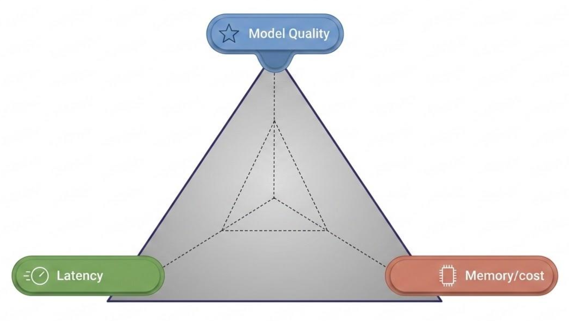
Model quality refers to the model’s predictive performance - accuracy, perplexity, and reasoning ability. Compression methods are fundamentally constrained by how much of this performance can be preserved after reducing parameters, precision, or computation. Most techniques (distillation, pruning, quantization) are evaluated first and foremost by how close they stay to the original model’s quality under a fixed budget.
Latency is determined not just by FLOPs but by memory bandwidth. At typical LLM inference batch sizes, the bottleneck is moving weights from GPU memory to compute units rather than performing arithmetic. This is why quantization has such outsized impact: INT4 reduces memory bandwidth usage by ~2× compared to INT8 and ~4× compared to FP32 (exact speedups depend on hardware and kernel support), which can reduce time-per-token in practice.
Speculative decoding also belongs in this latency axis. Instead of executing every token with the full model, a smaller draft model proposes multiple tokens which the large model verifies in parallel. When the draft is accurate, multiple tokens can be generated at close to the cost of a single large-model forward pass, reducing effective decoding steps and improving both latency and throughput. Its benefit depends strongly on draft quality and acceptance rate.
Memory/cost is the third axis and often the hard constraint in deployment. It includes both model weights and the KV cache, which grows with sequence length and batch size. This directly limits throughput because batch size is bounded by available memory. Techniques like GQA reduce KV cache size per token, while lower-precision KV storage (increasingly INT8 and sometimes INT4) further reduces memory pressure. Systems techniques like continuous batching and PagedAttention (a core component of vLLM) are orthogonal to model compression but compound with it by improving memory utilization and allowing more concurrent sequences within the same hardware budget.
The Pareto frontier - the set of models where improving one axis requires sacrificing another - has steadily moved toward better trade-offs over time, but it does not collapse. A model optimized for very low latency will always trade off some combination of quality or cost relative to one designed for higher throughput or accuracy. The engineering question is therefore not what is optimal in general, but which point on this frontier matches the deployment constraint.
A Concrete Example: From ResNet-50 to a Deployed Edge Classifier
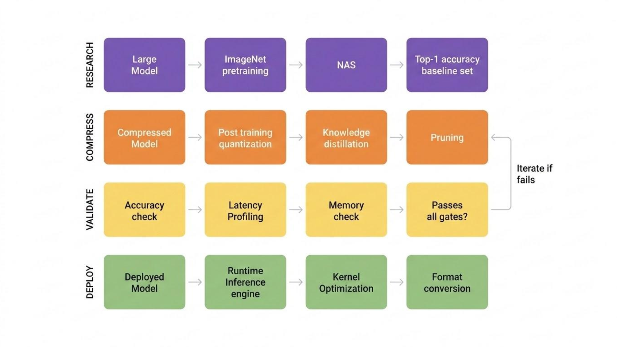
To make the pipeline concrete, consider the journey of an image classification model from research to deployment on an edge device such as a drone or smart camera. The process begins with ResNet-50, trained on ImageNet's 1.28 million images across 1,000 classes, achieving around 76% top-1 accuracy at 138 million parameters in FP32 - accurate but far too large and slow for edge deployment.
Rather than manually designing a smaller architecture, a NAS procedure such as MnasNet searches over candidate architectures by evaluating them directly on the target hardware, optimizing jointly for accuracy and measured latency. This produces a compact baseline tailored to the specific device rather than a general-purpose network adapted after the fact.
This architecture then enters the compression pipeline. Structured pruning removes low-magnitude filters, followed by knowledge distillation where the pruned model acts as a teacher to a MobileNetV2-style student - training against the teacher's soft probability distributions rather than hard labels alone, recovering accuracy that pruning alone would not achieve. Post-training quantization then converts weights from FP32 to INT8, typically with less than 1% accuracy drop for vision models at this scale.
The compressed model enters a validation gate - top-1 accuracy, milliseconds-per-image latency, and model size are each checked against deployment targets. If any gate fails, the pipeline iterates. Once all gates pass, the model is converted to TFLite, CoreML, or ONNX, with operator fusion and NPU-specific kernel optimizations applied. The result is a classifier running in real time on a camera or drone, at a fraction of the energy and memory of the original ResNet-50.
The Convergence
The trajectory across all these techniques points in the same direction. Architecture design established that the right mathematical primitives - depthwise separable convolutions, grouped attention, sparse routing - can eliminate orders of magnitude of unnecessary computation before any compression is applied. NAS automated the search for these primitives against real hardware constraints, removing human intuition as the bottleneck. Pruning revealed that trained networks are dramatically over-parameterized, and that much of their weight can be removed with surgical compensation rather than brute-force retraining. Distillation showed that the knowledge encoded in a large model is transferable - that a small model trained against a teacher's soft outputs learns a richer representation than one trained against labels alone. And quantization demonstrated that numerical precision is itself a design variable, one that can be traded against memory and bandwidth with surprisingly little loss when done carefully.
What has changed most fundamentally is not any single technique but the relationship between these techniques. They are no longer applied in isolation or as afterthoughts. Modern model development treats inference cost as a first-class constraint from the first design decision - architecture choices are validated for quantization robustness before training begins, distillation pipelines are built into the training recipe, and hardware-specific deployment targets shape the search space before a single parameter is learned. Compression is no longer something that happens to a model after research is done. It is part of what research means.
Learn more about how Union.ai enables model training at scale here.
References
- MobileNets (Howard et al., 2017)
- MobileNetV2 (Sandler et al., 2018)
- MobileNetV3 (Howard et al., 2019)
- Grouped Query Attention / GQA (Ainslie et al., 2023)
- Mistral 7B (Jiang et al., 2023)
- EfficientNet (Tan & Le, 2019)
- MnasNet (Tan et al., 2019)
- Once-for-All (Cai et al., 2020)
- Deep Compression (Han et al., 2015)
- The Lottery Ticket Hypothesis (Frankle & Carlin, 2019)
- SparseGPT (Frantar & Alistarh, 2023)
- Wanda (Sun et al., 2023)
- Knowledge Distillation (Hinton, Vinyals & Dean, 2015)
- DistilBERT (Sanh et al., 2019)
- TinyBERT (Jiao et al., 2020)
- DeiT (Touvron et al., 2021)
- GPTQ (Frantar et al., 2022)
- AWQ (Lin et al., 2023)
- BitNet b1.58 (Ma et al., 2024)
- Phi-3 (Abdin et al., 2024)
- Llama 3 / 3.2 (Meta, 2024)
- DeepSeek-V3 (DeepSeek, 2025)
- PagedAttention / vLLM (Kwon et al., 2023)
- Squeeze-and-Excitation Networks (Hu et al., 2018)