Biotech & Healthcare
Data Processing
Union.ai

From DNA to 3D Fold: Compare a Gene Across Six Species with Carbon and ESMFold

Sage Elliott

Sage Elliott

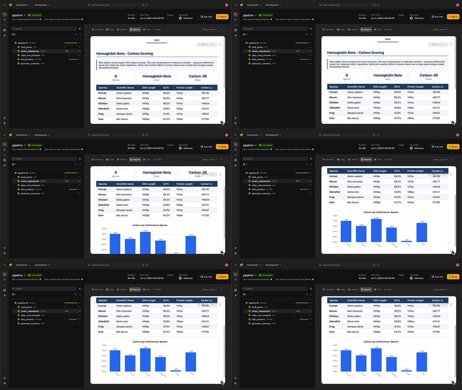
In this post we'll take a single gene, pull it from six species that diverged up to 450 million years ago, score the DNA with a language model, translate it to protein, fold it into 3D structures, and build a phylogenetic tree. One pipeline in pure Python. The key takeaway: protein structure is more conserved than sequence. Even when DNA changes significantly across species, the 3D fold often stays remarkably similar, because it's the shape, not the exact sequence, that keeps the organism alive. Until relatively recently, getting a 3D structure required months of wet-lab work per protein. Now Carbon and ESMFold let you run the same analysis across six species in minutes, turning what used to be a PhD project into a single pipeline run.

The full code is on GitHub. It runs on three curated gene sets (insulin, hemoglobin, p53) or any custom gene set you provide.
Why cross-species gene comparison matters

Every species on Earth shares a common ancestor, and we carry the proof in our DNA. The insulin gene in a human and a zebrafish diverged roughly 450 million years ago, but they're still recognizably the same gene. Insulin is so critical to survival that evolution can't change it much without killing the organism. For example fish insulin can still lower blood sugar in mammals.

This principle, that function constrains change, shows up everywhere in biology. But it shows up differently at different levels. DNA accumulates “silent” mutations (changes that don't alter the protein) freely, so DNA diverges faster than protein. And protein sequence diverges faster than protein structure, because many different sequences can fold into the same shape. Running the comparison across all three levels reveals how evolution actually works at the molecular level.

This isn't just academic. Understanding which parts of a gene are conserved tells drug designers which protein regions are functionally essential and likely to be similar across species, which matters for animal model selection and drug target validation. It tells geneticists which mutations are likely pathogenic (if the position is conserved, changing it is probably bad). And it gives computational biologists a way to validate their models: if your structure predictor shows the same fold across divergent species, it's probably capturing real biology.

The tools that make this analysis practical are recent. HuggingFace's Carbon is a DNA language model that scores how "natural" a sequence looks. Without it, you'd only be comparing raw sequence similarity, which treats every position equally. Carbon adds a learned signal: it can tell you that certain mutations matter more than others because they make the sequence look less like real DNA. That extra dimension helps distinguish functional divergence from neutral drift. Meta's ESMFold predicts 3D protein structure directly from the amino acid sequence. Combining them in a single pipeline gives you the full picture: DNA likelihood, sequence similarity, and structural comparison across species, all in one run.

Building the cross-species comparison pipeline

This is the kind of pipeline where AI orchestration pays off. Carbon-3B and ESMFold each need a GPU and significant memory, but loading gene sequences and building phylogenetic trees don't. Without proper AI orchestration, you either keep a GPU running the whole time (expensive) or manually shuffle data between scripts. Flyte lets you assign resources per task, so you only use (and pay for) a GPU when you're actually running a model. If ESMFold fails on a long protein (it can be memory-hungry), you can re-run from that step without re-scoring everything with Carbon. Every run is versioned, so when you're comparing results across gene sets or model versions, you can trace each result back to exactly what produced it. And the whole thing is pure Python: no YAML configs, no shell glue, no separate orchestration language.

The full code is on GitHub.

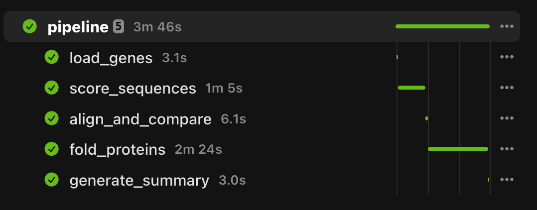
Five stages: load homologous gene sequences, score with Carbon, align sequences and compute pairwise similarity, fold proteins with ESMFold, generate an evolutionary summary.

Copied to clipboard!
Homologous   Carbon-3B    Needleman-     ESMFold      Summary
  Genes ──>  Scoring  ──>  Wunsch    ──> Folding ──>  Report
(6 species)     │         Alignment         │            │
                │            │              │            │
          Log-likelihood  DNA identity   3D structures  All metrics
          per species     Protein identity per species   + trees
                          Phylogenetic trees

Both environments are defined in `config.py`. The GPU environment gets 32Gi of memory to fit both Carbon-3B and ESMFold. The CPU environment is lightweight and handles data loading and summary generation. Flyte builds the container images from your requirements.txt list automatically, no separate Dockerfiles needed. 

Copied to clipboard!
# config.py

import flyte

base_image = flyte.Image.from_debian_base(
    name="genomic-gene-compare-v1",
).with_requirements("requirements.txt")

gpu_env = flyte.TaskEnvironment(
    name="genomic-gene-compare-gpu",
    image=base_image,
    resources=flyte.Resources(cpu=4, memory="32Gi", gpu=1),
)

cpu_env = flyte.TaskEnvironment(
    name="genomic-gene-compare-cpu",
    image=base_image,
    resources=flyte.Resources(cpu=2, memory="8Gi"),
)

The pipeline task orchestrates all five stages. Each `await` passes typed data between tasks. Flyte handles the serialization and transfer automatically. The pipeline returns both the comparison data and the structure data, so downstream analysis or visualization tools can consume either. We'll define each of the tasks called here in the sections that follow.
Copied to clipboard!
# workflow.py

@cpu_env.task(report=True)
async def pipeline(
    gene_set: str = "insulin",
    model_name: str = "HuggingFaceBio/Carbon-3B",
    custom_json: str = "",
) -> tuple[str, str]:

    # Stage 1: Load homologous gene sequences
    genes_dir = await load_genes(gene_set=gene_set, custom_json=custom_json)

    # Stage 2: Score with Carbon
    scores_json = await score_sequences(genes_dir=genes_dir, model_name=model_name)

    # Stage 3: Align sequences and compute pairwise similarity
    comparison_json = await align_and_compare(scores_json=scores_json, genes_dir=genes_dir)

    # Stage 4: Fold translated proteins with ESMFold
    structures_json = await fold_proteins(comparison_json=comparison_json)

    # Stage 5: Generate summary with phylogenetic trees
    summary_json = await generate_summary(
        comparison_json=comparison_json,
        structures_json=structures_json,
    )

    return comparison_json, structures_json

The gene sets

The pipeline ships with three curated gene sets, each chosen to show different evolutionary pressures. You can also pass your own sequences as custom JSON.

Copied to clipboard!
# workflow.py

GENE_SETS = {
    "insulin": {
        "gene_name": "Insulin",
        "description": "Insulin regulates blood sugar in all vertebrates. Highly conserved "
                       "across 500M+ years of evolution - even fish insulin can lower blood "
                       "sugar in humans.",
        "sequences": {
            "Human": {
                "dna": "ATGGCCCTGTGGATGCGCCTCCTGCCCCTGCTGGCGCTGCTGGCCCTCTGG...",
                "common_name": "Homo sapiens",
            },
            "Mouse": { ... },    # Mus musculus: diverged ~90M years ago
            "Chicken": { ... },  # Gallus gallu: diverged ~310M years ago
            "Zebrafish": { ... },# Danio rerio: diverged ~450M years ago
            "Frog": { ... },     # Xenopus laevis
            "Cow": { ... },      # Bos taurus: bovine insulin treated diabetics before recombinant
        },
    },
    "hemoglobin": { ... },  # Beta-globin: most studied gene in molecular evolution
    "p53": { ... },          # Tumor suppressor: elephant has 20 copies (Peto's paradox)
}

Each gene set tells a different story. Insulin is the textbook example of purifying selection: so critical that even fish and human versions can be “interchangeable”. Hemoglobin beta is one of the most studied genes in molecular evolution, and sequence differences between species power the "molecular clock" hypothesis that underpins modern phylogenetics. The p53 set is the most surprising: it includes an elephant, which has 20 copies of this tumor suppressor gene compared to our single copy. This may explain why elephants have extremely low cancer rates despite their massive body size, a puzzle known as Peto's paradox.

Understanding the biology: translation and sequence identity

Before diving into the pipeline tasks, it helps to understand the biology utilities that underpin the analysis. DNA is read in groups of three letters called codons. Each codon maps to one amino acid, and amino acids are the building blocks of proteins. The codon table below is that mapping. It's the key to understanding why protein is more conserved than DNA: the mapping is redundant. Four different codons all encode the same amino acid Leucine (CTT, CTC, CTA, CTG). A mutation that changes CTT to CTC changes the DNA but not the protein. These synonymous mutations accumulate freely over evolutionary time, which is why DNA diverges faster than protein for coding genes.

Copied to clipboard!
# workflow.py

CODON_TABLE = {
    "TTT": "F", "TTC": "F", "TTA": "L", "TTG": "L", "CTT": "L", "CTC": "L",
    "CTA": "L", "CTG": "L", "ATT": "I", "ATC": "I", "ATA": "I", "ATG": "M",
    "GTT": "V", "GTC": "V", "GTA": "V", "GTG": "V", "TCT": "S", "TCC": "S",
    "TCA": "S", "TCG": "S", "CCT": "P", "CCC": "P", "CCA": "P", "CCG": "P",
    "ACT": "T", "ACC": "T", "ACA": "T", "ACG": "T", "GCT": "A", "GCC": "A",
    "GCA": "A", "GCG": "A", "TAT": "Y", "TAC": "Y", "TAA": "*", "TAG": "*",
    "CAT": "H", "CAC": "H", "CAA": "Q", "CAG": "Q", "AAT": "N", "AAC": "N",
    "AAA": "K", "AAG": "K", "GAT": "D", "GAC": "D", "GAA": "E", "GAG": "E",
    "TGT": "C", "TGC": "C", "TGA": "*", "TGG": "W", "CGT": "R", "CGC": "R",
    "CGA": "R", "CGG": "R", "AGT": "S", "AGC": "S", "AGA": "R", "AGG": "R",
    "GGT": "G", "GGC": "G", "GGA": "G", "GGG": "G",
}


def _translate(dna: str) -> str:
    """Translate DNA to protein in reading frame 0."""
    dna = dna.upper()
    protein = []
    for i in range(0, len(dna) - 2, 3):
        codon = dna[i:i + 3]
        aa = CODON_TABLE.get(codon, "X")
        if aa == "*":
            break
        protein.append(aa)
    return "".join(protein)


def _gc_content(seq: str) -> float:
    if not seq:
        return 0.0
    return sum(1 for b in seq.upper() if b in "GC") / len(seq)


def _sequence_identity(seq1: str, seq2: str, match: int = 2, mismatch: int = -1, gap: int = -2) -> float:
    """Percent identity via Needleman-Wunsch global alignment."""
    if not seq1 or not seq2:
        return 0.0
    n, m = len(seq1), len(seq2)

    # Build score matrix
    dp = [[0] * (m + 1) for _ in range(n + 1)]
    for i in range(1, n + 1):
        dp[i][0] = dp[i - 1][0] + gap
    for j in range(1, m + 1):
        dp[0][j] = dp[0][j - 1] + gap
    for i in range(1, n + 1):
        for j in range(1, m + 1):
            s = match if seq1[i - 1] == seq2[j - 1] else mismatch
            dp[i][j] = max(dp[i - 1][j - 1] + s, dp[i - 1][j] + gap, dp[i][j - 1] + gap)

    # Traceback to count matches and alignment length
    i, j = n, m
    matches = 0
    aligned = 0
    while i > 0 or j > 0:
        if i > 0 and j > 0:
            s = match if seq1[i - 1] == seq2[j - 1] else mismatch
            if dp[i][j] == dp[i - 1][j - 1] + s:
                if seq1[i - 1] == seq2[j - 1]:
                    matches += 1
                aligned += 1
                i -= 1
                j -= 1
                continue
        if i > 0 and dp[i][j] == dp[i - 1][j] + gap:
            aligned += 1
            i -= 1
        else:
            aligned += 1
            j -= 1

    return matches / aligned if aligned else 0.0

The `_translate` function reads DNA in triplets (codons) and converts each to an amino acid, stopping at a stop codon (*). The `_gc_content` function measures the proportion of G and C bases, which varies between species and can affect how DNA language models score sequences. The `_sequence_identity` function uses Needleman-Wunsch global alignment, a standard algorithm in bioinformatics for comparing two sequences. It inserts gaps to find the optimal alignment, then computes identity as matches divided by aligned length. This handles the real-world case where homologous proteins differ in length (e.g., cow hemoglobin beta is 145 aa while human is 147 aa), a naive position-by-position comparison would show near-zero identity due to the offset, while Needleman-Wunsch correctly reports ~84%.

Task 1: Load homologous gene sequences

The first task is simple but important. It loads one of the curated gene sets or accepts custom JSON, and outputs a directory that the rest of the pipeline consumes. The `cache="auto"` decorator means switching between gene sets is instant after the first run. When you're comparing insulin, hemoglobin, and p53 in sequence, only the first load for each gene set actually executes.

Copied to clipboard!
# workflow.py

@cpu_env.task(cache="auto")
async def load_genes(
    gene_set: str = "insulin",
    custom_json: str = "",
) -> flyte.io.Dir:
    if custom_json:
        data = json.loads(custom_json)
    elif gene_set in GENE_SETS:
        data = GENE_SETS[gene_set]
    else:
        available = ", ".join(GENE_SETS.keys())
        raise ValueError(f"Unknown gene set '{gene_set}'. Available: {available}")

    out_dir = tempfile.mkdtemp(prefix="gene_compare_")
    with open(os.path.join(out_dir, "genes.json"), "w") as f:
        json.dump(data, f)

    return await flyte.io.Dir.from_local(out_dir)

Task 2: Score DNA with Carbon

Carbon-3B is a DNA language model trained on genomic sequences. It scores each species' DNA for log-likelihood, essentially a probability score for the sequence. A higher log-likelihood means the sequence looks more "natural" to the model, similar to how a language model would rate "the cat sat on the mat" higher than a random string of words. This task focuses purely on scoring, the sequence comparison comes in the next step.

Copied to clipboard!
# workflow.py
@gpu_env.task(report=True)
async def score_sequences(
    genes_dir: flyte.io.Dir,
    model_name: str = "HuggingFaceBio/Carbon-3B",
) -> str:
    import torch
    from transformers import AutoModelForCausalLM, AutoTokenizer

    device = "cuda" if torch.cuda.is_available() else "cpu"

    tokenizer = AutoTokenizer.from_pretrained(model_name, trust_remote_code=True)
    model = AutoModelForCausalLM.from_pretrained(
        model_name, trust_remote_code=True,
        dtype=torch.bfloat16 if device == "cuda" else torch.float32,
    ).to(device)
    model.eval()

    genes_path = await genes_dir.download()
    with open(os.path.join(genes_path, "genes.json")) as f:
        data = json.load(f)

    species_names = list(data["sequences"].keys())

    scores = {}
    for i, species in enumerate(species_names):
        dna = data["sequences"][species]["dna"]
        prompt = f"<dna>{dna}"
        inputs = tokenizer(prompt, return_tensors="pt", add_special_tokens=False).to(device)

        with torch.no_grad():
            output = model(**inputs, labels=inputs["input_ids"])
            loss = output.loss.item()
            ll = -loss * inputs["input_ids"].shape[1]

        protein = _translate(dna)
        scores[species] = {
            "log_likelihood": round(ll, 4),
            "loss": round(loss, 4),
            "gc_content": round(_gc_content(dna), 4),
            "length": len(dna),
            "protein": protein,
            "protein_length": len(protein),
            "common_name": data["sequences"][species]["common_name"],
        }

    result = {
        "gene_name": data["gene_name"],
        "description": data["description"],
        "species": species_names,
        "scores": scores,
    }
    return json.dumps(result)

The `<span>&lt;dna></span>` prefix tells the model to interpret the input as a DNA sequence rather than text. The loss is the average negative log-likelihood per token; multiplying by sequence length gives the total log-likelihood for the full sequence. Species whose DNA looks more "natural" to the model (higher log-likelihood) may have sequences closer to what Carbon saw in its training data, which skews toward well-studied model organisms like humans and mice. This is interesting in itself: the model's confidence can vary across species in ways that reflect how much genomic data exists for each organism.

Task 3: Align sequences and compute cross-species similarity
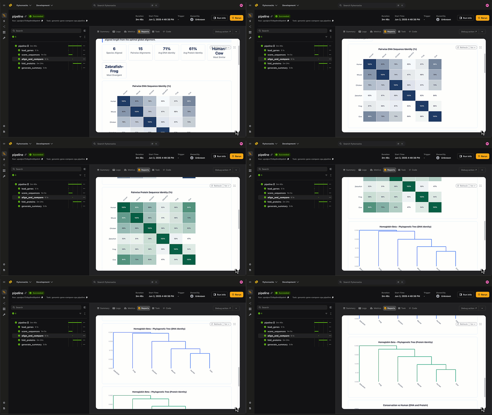
This is where the cross-species comparison happens. The task runs Needleman-Wunsch global alignment on every pair of species, at both the DNA and protein level. Pairwise means comparing every species against every other species, and identity is the percentage of matching positions in the optimal alignment. The result is two grids (one for DNA, one for protein) that show how similar each pair of species is at the molecular level, plus phylogenetic trees built from the divergence.

Comparing the two grids is where the insight comes from: if protein identity is much higher than DNA identity for a gene, that means evolution is changing the DNA but preserving the protein. That's direct evidence the protein's function is under selective pressure.

This task runs on CPU since it's pure computation, no deep learning models needed. Separating it from the GPU-bound Carbon scoring means you only pay for GPU time when you're actually running a model.

Copied to clipboard!
# workflow.py

@cpu_env.task(report=True)
async def align_and_compare(
    scores_json: str,
    genes_dir: flyte.io.Dir,
) -> str:
    scores_data = json.loads(scores_json)
    species_names = scores_data["species"]
    scores = scores_data["scores"]

    genes_path = await genes_dir.download()
    with open(os.path.join(genes_path, "genes.json")) as f:
        data = json.load(f)

    # Pairwise DNA identity matrix
    identity_matrix = []
    for sp1 in species_names:
        row = []
        for sp2 in species_names:
            dna1 = data["sequences"][sp1]["dna"]
            dna2 = data["sequences"][sp2]["dna"]
            identity = _sequence_identity(dna1, dna2)
            row.append(round(identity, 4))
        identity_matrix.append(row)

    # Pairwise protein identity matrix
    protein_matrix = []
    for sp1 in species_names:
        row = []
        for sp2 in species_names:
            identity = _sequence_identity(scores[sp1]["protein"], scores[sp2]["protein"])
            row.append(round(identity, 4))
        protein_matrix.append(row)

    result = {
        "gene_name": scores_data["gene_name"],
        "description": scores_data["description"],
        "species": species_names,
        "scores": scores,
        "dna_identity_matrix": identity_matrix,
        "protein_identity_matrix": protein_matrix,
    }
    return json.dumps(result)

The identity matrices are the core comparison output. The gap between DNA and protein identity is the evolutionary signal: when protein identity is significantly higher than DNA identity, synonymous mutations are accumulating while the protein stays conserved. That's purifying selection in action, and it's the central biological insight this pipeline reveals.

Task 4: Fold proteins with ESMFold for 3D structure comparison
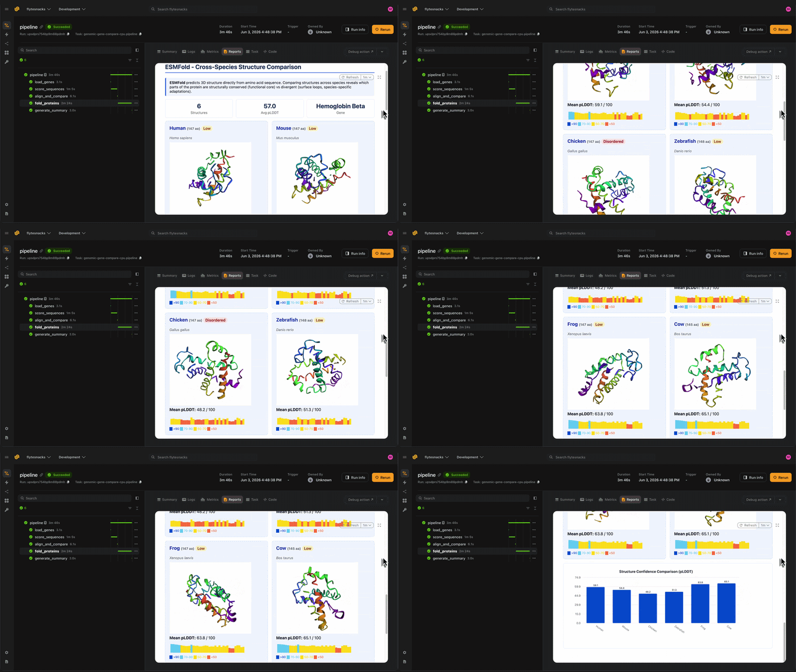
Sequence comparison tells you how much the gene has changed. Structure comparison tells you whether those changes actually matter. ESMFold predicts 3D protein structure directly from amino acid sequence, no multiple sequence alignment needed. By folding the same gene's protein from each species, we can see whether sequence divergence translates to structural divergence, or whether the fold is preserved despite the surface-level changes.

Copied to clipboard!
# workflow.py


@gpu_env.task(report=True)
async def fold_proteins(
    comparison_json: str,
    max_length: int = 400,
) -> str:
    import torch
    import numpy as np
    from transformers import AutoTokenizer, EsmForProteinFolding

    comparison = json.loads(comparison_json)
    species_names = comparison["species"]
    scores = comparison["scores"]

    device = "cuda" if torch.cuda.is_available() else "cpu"

    tokenizer = AutoTokenizer.from_pretrained("facebook/esmfold_v1")
    model = EsmForProteinFolding.from_pretrained("facebook/esmfold_v1", low_cpu_mem_usage=True)
    model = model.to(device)
    model.eval()

    structure_data = {}

    for idx, species in enumerate(species_names):
        protein = scores[species]["protein"]

        if len(protein) > max_length:
            continue

        inputs = tokenizer(protein, return_tensors="pt", add_special_tokens=False).to(device)

        with torch.no_grad():
            outputs = model(**inputs)

        pdb_str = _outputs_to_pdb(outputs, protein)

        plddt_raw = outputs.plddt[0].cpu().numpy()
        if plddt_raw.ndim == 2:
            plddt_raw = plddt_raw[-1]
        plddt = plddt_raw.flatten()[:len(protein)]
        if plddt.max() <= 1.0:
            plddt = plddt * 100
        plddt_mean = float(np.mean(plddt))

        structure_data[species] = {
            "pdb_str": pdb_str,
            "plddt_mean": round(plddt_mean, 1),
            "plddt_per_residue": [round(float(v), 1) for v in plddt[:len(protein)]],
            "protein_length": len(protein),
        }

    return json.dumps(structure_data)

The `max_length=400` parameter is a practical constraint. ESMFold's memory usage scales quadratically with sequence length, so longer proteins can run out of GPU memory. The gene sets in this tutorial use full-length coding sequences: insulin is ~105-110 residues, hemoglobin ~145-148, and p53 ~367-393, all within the limit. If you bring your own gene set with longer proteins, you may need to increase GPU memory or raise the limit.

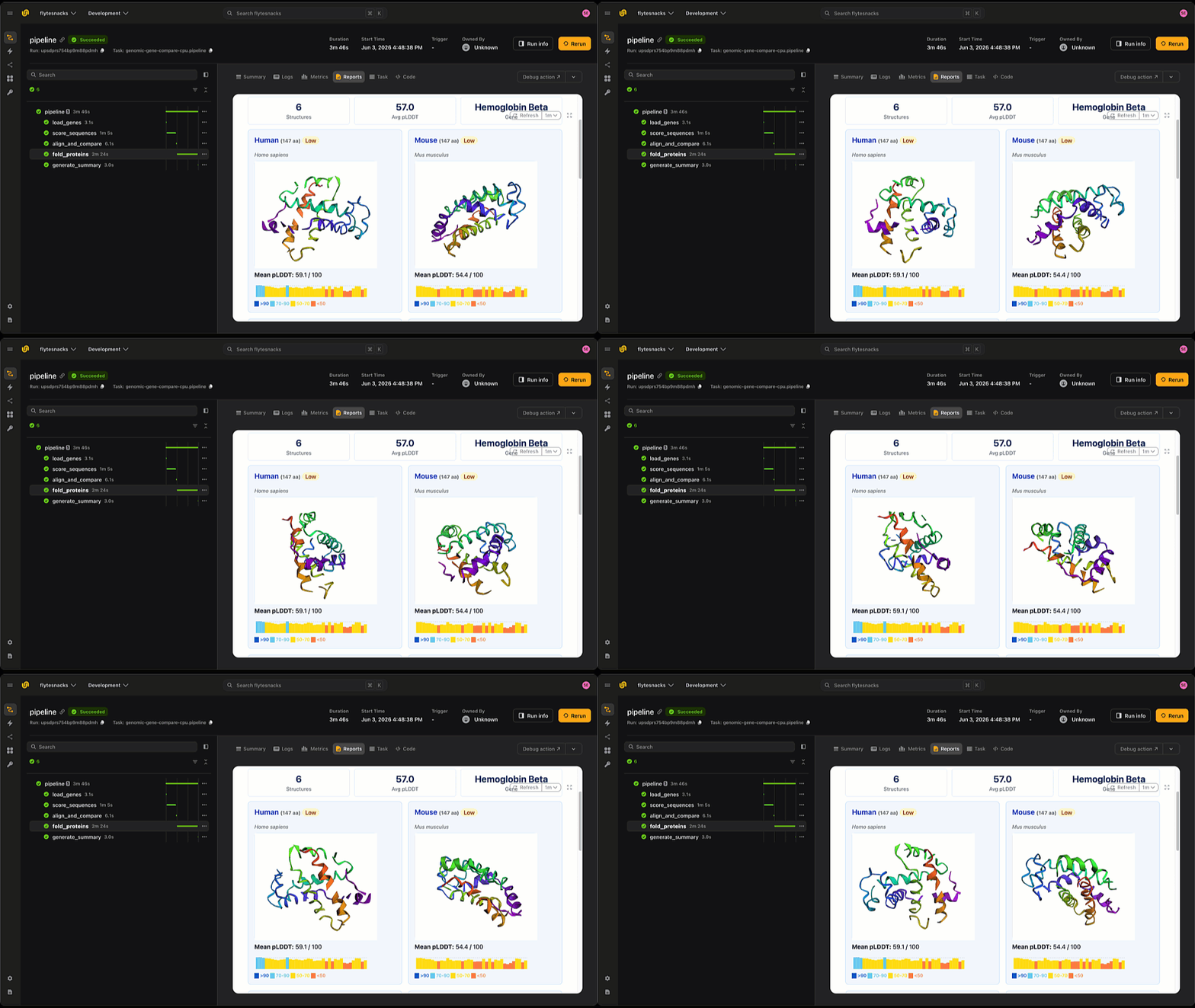
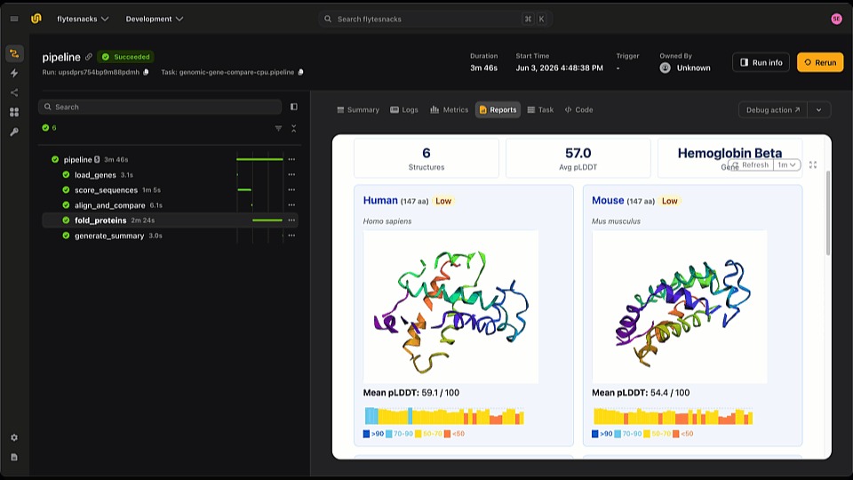
The PDB (Protein Data Bank) conversion function transforms ESMFold's predicted atom coordinates into standard PDB format. The Flyte report renders these as interactive 3D viewers using 3Dmol.js, so you can spin and zoom the structures directly in the Flyte dashboard.

Copied to clipboard!
# workflow.py

def _outputs_to_pdb(outputs, sequence: str) -> str:
    import numpy as np

    pos = outputs.positions[0]
    if pos.dim() == 4:
        pos = pos[-1]
    positions = pos.cpu().numpy()
    atom_names = ["N", "CA", "C", "O"]
    aa_3letter = {
        "A": "ALA", "R": "ARG", "N": "ASN", "D": "ASP", "C": "CYS",
        "Q": "GLN", "E": "GLU", "G": "GLY", "H": "HIS", "I": "ILE",
        "L": "LEU", "K": "LYS", "M": "MET", "F": "PHE", "P": "PRO",
        "S": "SER", "T": "THR", "W": "TRP", "Y": "TYR", "V": "VAL",
    }

    pdb_lines = []
    atom_idx = 1
    for res_idx, aa in enumerate(sequence):
        res_name = aa_3letter.get(aa, "UNK")
        for atom_i, atom_name in enumerate(atom_names):
            if atom_i >= positions.shape[1]:
                break
            x, y, z = positions[res_idx, atom_i]
            if any(math.isnan(c) for c in (x, y, z)):
                continue
            pdb_lines.append(
                f"ATOM  {atom_idx:5d}  {atom_name:<3s} {res_name} A{res_idx + 1:4d}    "
                f"{x:8.3f}{y:8.3f}{z:8.3f}  1.00  0.00           {atom_name[0]:>2s}"
            )
            atom_idx += 1
    pdb_lines.append("END")
    return "\n".join(pdb_lines)

The pLDDT (predicted Local Distance Difference Test) score is ESMFold's per-residue confidence measure. Above 90 means very high confidence, typically the structured core of the protein. Between 70-90 is confident. Between 50-70 suggests flexible loops or less certain regions. Below 50 usually indicates disorder, meaning that part of the protein doesn't adopt a fixed shape. Comparing pLDDT across species can reveal which structural regions are consistently well-folded (likely functionally important) versus which regions are more variable.

Task 5: Generate evolutionary summary
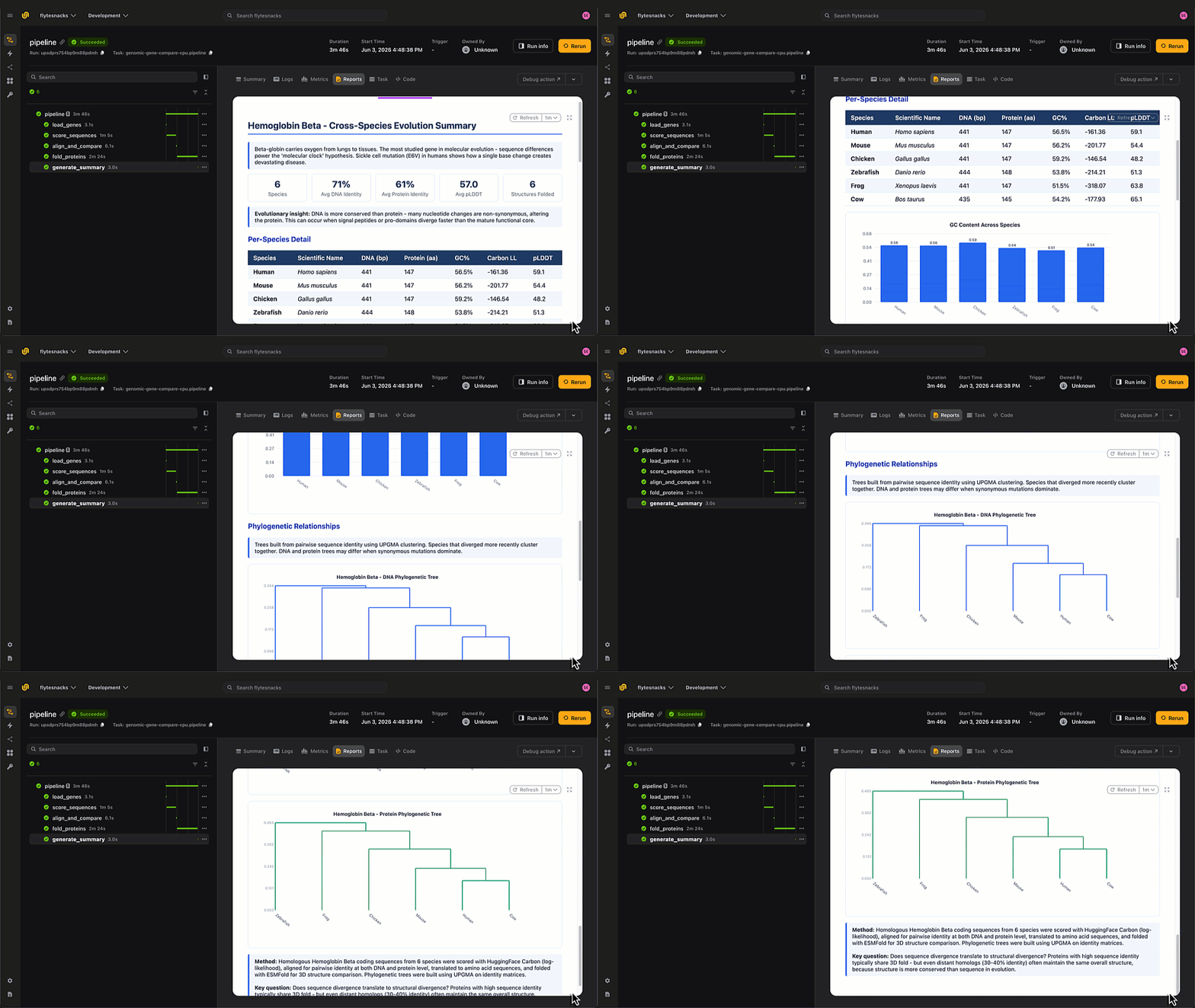
The final task brings everything together. It computes cross-species statistics, builds phylogenetic trees from both identity matrices, and produces a consolidated summary report. This task runs on CPU since it's pure computation, no models needed.

Copied to clipboard!
# workflow.py

@cpu_env.task(report=True)
async def generate_summary(
    comparison_json: str,
    structures_json: str,
) -> str:
    comparison = json.loads(comparison_json)
    structures = json.loads(structures_json)

    species = comparison["species"]
    scores = comparison["scores"]
    gene_name = comparison["gene_name"]
    dna_matrix = comparison["dna_identity_matrix"]
    protein_matrix = comparison["protein_identity_matrix"]

    # Average pairwise identity (exclude diagonal)
    n = len(species)
    dna_pairs = [dna_matrix[i][j] for i in range(n) for j in range(i + 1, n)]
    protein_pairs = [protein_matrix[i][j] for i in range(n) for j in range(i + 1, n)]
    avg_dna_id = sum(dna_pairs) / len(dna_pairs) if dna_pairs else 0
    avg_protein_id = sum(protein_pairs) / len(protein_pairs) if protein_pairs else 0
    avg_plddt = sum(d["plddt_mean"] for d in structures.values()) / len(structures) if structures else 0

    summary = {
        "gene_name": gene_name,
        "n_species": n,
        "avg_dna_identity": round(avg_dna_id, 4),
        "avg_protein_identity": round(avg_protein_id, 4),
        "avg_plddt": round(avg_plddt, 1),
        "n_structures": len(structures),
    }
    return json.dumps(summary)

The phylogenetic trees are built from the identity matrices using UPGMA (Unweighted Pair Group Method with Arithmetic Mean) clustering. The pipeline includes a full UPGMA implementation and SVG dendrogram renderer (in the full source) that converts the pairwise distances into a tree showing which species are most closely related at the molecular level. An interesting result: DNA trees and protein trees can differ for the same gene when synonymous mutations dominate, because the DNA has diverged further than the protein it encodes.

Every run in Flyte is versioned, so you can compare results across different gene sets or different Carbon model versions and trace each result back to exactly what inputs produced it.

Running the pipeline

This will run on your flyte on your cluster which needs a GPU (recommended for ESMFold), but you can also run locally. 

Default (Insulin across 6 species):

Copied to clipboard!
flyte run workflow.py pipeline --gene_set "insulin"

Hemoglobin comparison:

Copied to clipboard!
flyte run workflow.py pipeline --gene_set "hemoglobin"

p53, including elephant:

Copied to clipboard!
flyte run workflow.py pipeline --gene_set "p53"

Run Locally 

The same code runs locally and remotely. Flyte handles the GPU scheduling, container builds, and data transfer between tasks. Locally you can test with the TUI for a live terminal dashboard. Remotely, the Flyte UI shows interactive reports with identity heatmaps, phylogenetic dendrograms, and spinning 3D protein structures.

Copied to clipboard!
flyte run --local --tui workflow.py pipeline --gene_set "hemoglobin"

What’s next

The tutorial ships with three gene sets, but the pipeline accepts custom JSON so you can compare any set of homologous genes. Grab orthologous sequences from Ensembl or NCBI Orthologs, format them as a JSON object matching the gene set structure, and pass them via `--custom_json`. There are also two companion tutorials in the workshops repo: genomic-variant-effect for mutation impact analysis and genomic-dna-generation for DNA generation with Carbon.

Check out the full code on GitHub to run on Flyte or Union and try it with your own gene sets.
Try the devbox

A free, local sandbox to explore the Union.ai platform.

Chat with an engineer
No items found.